[논문리뷰] SimCLR: A Simple Framework for Contrastive Learning of Visual Representations (ICML ‘20)

12 Nov 2022 in Papers / Review

논문도 잘 읽히고, 직관적이며 다양한 실험이 있어서 읽으면 좋은 논문이라고 생각합니다.

저자들이 주장하는 SimCLR의 contribution은 다음과 같습니다.

• Data augmentation을 framework에 적용한 predictive task 정의
• Representation과 contrastive loss 사이에 학습 가능한 비선형 transformation 적용
• Contrastive learning이 잘되려면 큰 batch size와 긴 train epoch 필요

---

1. Introduction

사람이 정의한 supervision (label) 없이 visual representation을 학습하는 방식은 크게 2가지로 나눌 수 있습니다.

• Generative approach

  • 단점 : Pixel-level generation의 연산 cost가 높다.

• Discriminative approach

  • 단점 : Pretext task를 정의하는 과정에서 heuristic에 의존하게 된다. (pretext task : 사람이 정의한 representation 학습 방법)
  • 최근 latent space에 contrastive learning을 적용하여 SOTA 결과를 얻었다.

저자들은 discriminative approach에 contrastive learning을 적용하는 간단한 framework인 SimCLR을 제안합니다.

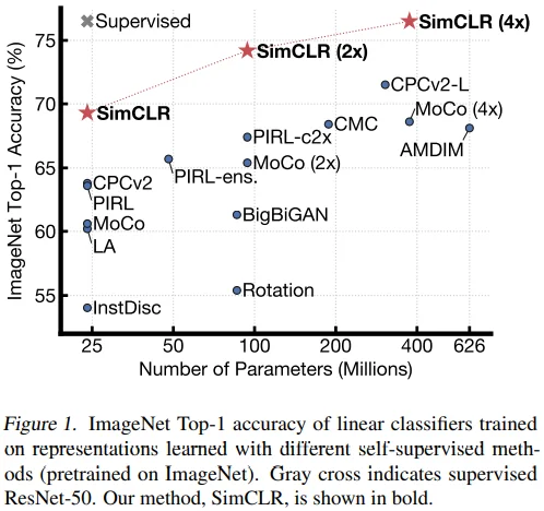
SimCLR은 Figure 1에서 볼 수 있듯 다른 연구에 비해 높은 score를 기록했을 뿐 아니라, 매우 간단한 구조로 작동하며, (이전의 연구들에서 사용했던 memory 부담이 있는) memory bank가 필요없다는 장점이 있습니다.

저자들이 실험을 통해 밝힌 내용은 다음과 같습니다.

• Contrastive prediction task를 정의함에 있어서, multiple data augmentation이 중요한 역할을 한다.
• Representation과 contrastive loss 사이에 학습 가능한 비선형 transformation을 적용하면, representation을 더 잘 학습할 수 있다.
• Contrastive cross entropy loss 사용 시, normalized embedding과 temperature parameter가 중요한 역할을 한다.
• Contrastive learning은 supervised learning보다 큰 batch size와 긴 train time이 필요하며, deeper and wider network를 사용할 때 더 잘 학습한다.

---

2. Method

2.1. The Contrastive Learning Framework

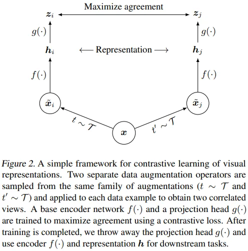
Figure 2를 통해 SimCLR framework를 설명하고 있으며, 아래 순서대로 적용됩니다.

• Data augmentation module

  • 이미지에 2개의 augmentation을 각각 적용하여 그 결과를 positive pair로 간주합니다.

  • 적용되는 augmentation은 크게 3종류입니다.

    • Random crop > resize back to origin size
    • Random color distortion
    • Random Gaussian blur

• Base encoder

  • Augmented image로부터 representation vector를 추출하기 위한 network로, network의 종류에 구애받지 않습니다.
  • SimCLR에서는 ResNet을 사용했습니다.

• Projection head

  • Representation vector를 contrastive loss가 적용되는 차원으로 mapping하는 network입니다.
  • SimCLR에서는 Linear - BN - ReLU - Linear - BN 구조의 MLP를 사용했습니다.

• Contrastive loss function

  • N개의 mini-batch에 augmentation을 각각 적용하여 image (2N)개를 얻게 됩니다.
  • 하나의 이미지로부터 얻어진 augmented image 2개를 positive pair로 간주하고, 이외의 이미지 (2N-2)개를 negative pair로 간주합니다.

  • Positive pair (i,j)에 대한 loss function은 다음과 같습니다. ($l_{i,j} \not = l_{j,i}$)

    • \[\begin{equation} l_{i,j} = -log \frac {exp(sim(z_i, z_j)/\tau)} {\sum^{2N}_{k=1} {\mathbb I}_{[k \not = i]} exp(sim(z_i, z_k)/\tau)} , \tag{1}\end{equation}\]
    • ${\mathbb I}_{[k \not = i]}$ : Indicator function evaluating to 1 iff $k \not = i$
    • $\tau$ : temperature parameter
    • $sim(u, v) = \frac {w^{\intercal}v} {|u||v|}$ : the dot product between $l_2$ normalized $u$ and $v$ (i.e. cosine similarity)
    • SimCLR 저자들은 이를 NT-Xent loss (the normalized temperature-scaled cross entropy loss)로 부릅니다.

2.2. Training with Large Batch Size

• 이전의 연구에서 사용했던 memory bank를 사용하는 대신 batch size를 8192까지 늘렸습니다.

  • Memory bank : Unsupervised Feature Learning via Non-Parametric Instance-level Discrimination (Wu et al. 2018)

• 큰 batch size에서의 안정적인 학습을 위해 LARS optimizer를 사용했습니다.

  • LARS(Layer-wise Adaptive Rate Scaling) : Large Batch Training of Convolutional Networks (You et al. 2017)

Global BN

Information leakage를 막기 위해, 분산 학습 과정에서 모든 device에 대한 BN의 평균과 분산을 한번에 업데이트했습니다.

2.3. Evaluation Protocol

Datasets

• ImageNet

• CIFAR-10

  • Appendix B.9. CIFAR-10

    • ImageNet에서 얻은 결과가 CIFAR-10에서도 얻어지는지 확인하기 위해 사용했습니다.

    • ImageNet보다 image size가 작기 때문에 다음의 조치를 취했습니다.

      • Replace : First 7x7 Conv of stride 2 -> 3x3 Conv of stride 1
      • Remove : First max pooling layer
• Others for transfer learning

Metrics

Linear evaluation protocol

• Representation이 잘 학습되었는지 평가하기 위해 널리 사용된다고 합니다.
• Base encoder를 freeze한 이후 새로운 linear classifier를 학습시키는 방식으로, test accuracy를 representation quality로 간주합니다.

Defalut Setting

• Augmentation

  • Random crop + resize to origin size + random flip
  • Random color distortion
  • Random Gaussian blur

  • Appendix A. Data Augmentation Details

    • Inception-style random cropping

      • Random size : uniform from 0.08 to 1.0 in area
      • Random aspect ratio : from 3/4 to 4/3
• Base encoder : ResNet-50
• Projection head : Linear - BN - ReLU - Linear - BN (out dimension : 128)
• Criterion : NT-Xent loss
• Optimizer : LARS
• Learning rate : 4.8 (= 0.3 * batch_size / 256)
• Weight decay : $10^{-6}$
• Batch size : 4096 (for 100 epochs)
• Linear warmup for the first 10 epochs
• Cosine decay schedule without restarts

---

3. Data Augmentation for Contrastive Representation Learning

Data augmentation defines predictive tasks

Representation learning을 위해 data augmentation을 널리 사용해왔지만, 지금까지는 network architecture의 변화를 통해 contrastive prediction task를 수행하고자 했습니다.

• Network architecture 상에서 receptive field를 제한하여 global-to-local view prediction 수행
• Context aggregattion network로 image patch에 대한 neighboring view prediction 수행

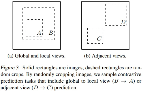
저자들은 random crop과 같은 augmentation을 통해 위의 task를 간단하게 해결할 수 있다고 주장합니다.

• Figure 3을 보면 image에 augmentation을 적용해 얻어낸 2개의 image가 어떤 관계로 해석될 수 있는지를 보여주고 있습니다. 이는 마치 앞선 연구에서 수행하고자 했던 global-local-view prediction과 neighboring view prediction task를 수행한다고 볼 수 있습니다. 즉, 앞선 연구들과 다르게 SimCLR을 적용하면 contrastive prediction task를 해결하기 위해 network architecture를 바꿀 필요가 없어진다는 장점이 있습니다.

3.1. Composition of data augmentation operations is crucial for learning good representations

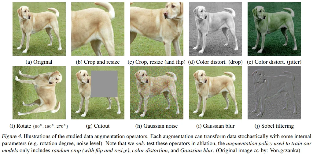
Figure 4는 실험에 사용한 augmentation을 보여주고 있습니다.

• Spatial/geometric transformation

  • Crop
  • Resize (with horizontal flip)
  • Rotation
  • CutOut

• Appearance transformation

  • Color distortion (Color drop, brightness, contrast, saturation, hue)
  • Gaussian blur
  • Sobel filtering

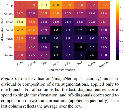
Figure 5에서 Linear evaluation 방식으로 augmentation의 성능을 평가했습니다. 참고로, ImageNet은 제각기 다른 image size를 갖기 때문에 crop이 필요한 경우 원본 이미지에 crop과 resize를 먼저 적용했습니다. 이후 다른 augmnetation을 적용함으로써, model 성능의 하락이 예상되긴 하지만 공정한 평가가 될 수 있도록 했습니다.

이해를 돕기 위한 예시는 다음과 같습니다. (뇌피셜)

• (Crop, Crop) : Crop 1개만 적용하는 것과 동일
• (Crop, Color) : Random crop + resize 적용 -> 2개의 이미지에 각각 identity, color distortion 적용
• (Color, Crop) : 1개의 이미지에 먼저 color distortion 적용 -> color distortion이 적용된 이미지와 원본 이미지 모두 동일한 random crop + resize 적용

흥미로운 점은 하나의 augmentation만 적용했을 때 contrastive task 상의 positive pair를 완벽히 학습했음에도 성능이 좋지 않았다고 합니다. 하지만 2개의 augmentation을 각각 적용하여 contrastive prediction task를 어렵게 만들었을 때 representation의 성능이 매우 좋아졌습니다. 여러 조합 중에서 특히 (Crop, Color), (Color, Crop) 조합의 성능이 특히 높은 것을 볼 수 있습니다.

• Appendix B.2. Broader composition of data augmentations further improves performance

  • Broader data augmentations (Equalize, Solarize, Motion blur)를 적용하여, linear evaluation 성능이 소폭 상승했습니다.

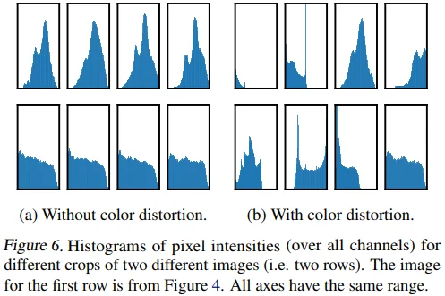
저자들은 color distortion 여부에 따른 pixel histogram을 Figure 6로 보여줍니다.

• (a)를 보면, color distortion이 없을 경우 random crop을 한다고 하더라도 crop 결과의 pixel histogram이 유사한 것을 볼 수 있습니다.
• 반면, (b)에서는 각각의 crop에 대한 histogram이 제각기 다른 것을 볼 수 있습니다.
• 즉, model이 올바른 representation을 학습하기 보다는 (상대적으로 쉬운) color에 편향된 방향으로 학습할 여지가 있고, 그렇기 때문에 crop과 color distortion을 같이 사용하는 것이 매우 중요하다는 결론을 내릴 수 있습니다.

3.2. Contrastive learning needs stronger data augmentation than supervised learning

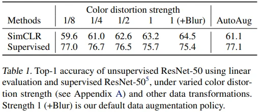
• Table 1을 보면 color distortion의 strength를 높일수록, simCLR로 학습된 model의 linear evaluation 성능은 향상되었지만, supervised learning으로 학습된 model에서는 오히려 성능이 하락하는 것을 볼 수 있습니다.
• 반면, color distortion이 아니라 AutoAugment를 적용했을 때는 성능 향상/하락이 반대되는 것을 볼 수 있습니다.
• 즉, color distortion을 강하게 하는 것이 contrastive learning에 매우 효과적임을 밝혔고, AutoAugment와의 비교를 통해 이러한 성능 향상이 단순히 augmentation으로 인한 것이 아님을 보였습니다.

---

4. Architectures for Encoder and Head

4.1. Unsupervised contrastive learning benefits (more) from bigger models

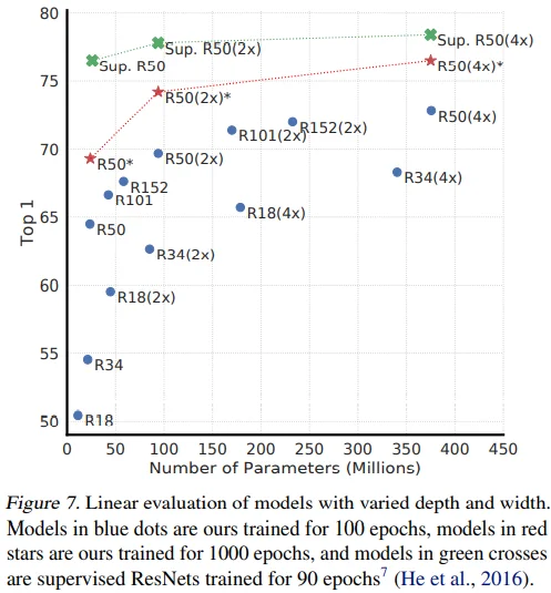
Figure 7을 통해 supervised learning과 마찬가지로 contrastive learning model의 depth와 width에 성능이 비례하며, model 크기가 커질수록 supervised learning에 비해 contrastive learning의 성능 향상 폭이 증가하는 것을 볼 수 있습니다.

• Appendix B.3. Effects of Longer Training for Supervised Models

  • Supervised model의 train epoch를 키운다거나 더 강한 augmentatation을 적용하더라도 일관된 유의미한 결과는 없었습니다.

4.2. A nonlinear projection head improves the representation quality of the layer before it

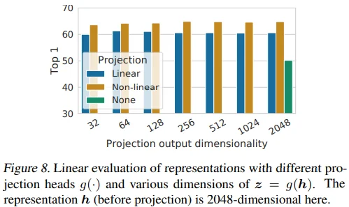
Figure 8은 적절한 projection head를 찾기 위한 실험으로, head 종류 3가지와 함께 최적의 output dimension을 찾고자 했습니다.

• None = Identity mapping
• representation dimension = 2048
• 흥미로운 점은 projection output dim.과 linear evaluation 성능이 무관하다는 점입니다.
• 또한, 비선형 head > 선형 head >> None 관계를 확인할 수 있습니다. 이에 대해 저자들은 contrastive loss에 의해 정보를 잃어버릴 수 있기 때문에 representation 이후 비선형 projection을 사용하는 것이 중요하다는 가설을 세웠습니다. 특히, projection은 data augmentation과 무관하므로, downstream task에 유용할 수 있는 color, orientation 같은 정보를 지울 수 있다는 것입니다.

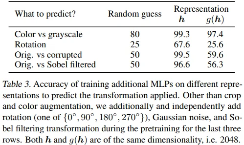
위 가설을 검증하기 위해 저자들은 추가 실험을 진행합니다. Pretraining 과정에 사용한 trasnformation을 예측하도록 model을 학습시켜 $h$와 $g(h)$ 중 어떤 representation이 더 많은 transformation 정보를 갖는지 비교했습니다. 그 결과는 Table 3에서 확인할 수 있습니다.

• $h$와 $g(h)$는 동일한 dimension을 갖고, $g$는 비선형 projection입니다.

• Color 예측에서는 2.1로 성능에 큰 차이가 없었지만, rotation (42.0), corruption (39.9), sobel (40.3)에서 차이가 컸고, $g(h)$가 random guess와 비교하여 별 차이가 없다는 것을 볼 수 있습니다. 즉, 비선형 projection을 적용했을 때, 학습에 사용했던 trasnformation 정보가 $h$ representation에 잘 보존되어 있다고 할 수 있습니다.

• Appendix B.4. Understanding The Non-Linear Projection Head

  • Linear projection matrix의 eigenvalue 분포를 시각화했을 때, 대부분이 낮은 값을 갖는 low-rank에 가까운 것을 확인할 수 있습니다. (뇌피셜 : 선형 projection head를 사용하면, representation의 일부 정보만 활용한다고 해석할 수도 있을 것 같습니다.)
  • T-SNE 시각화를 했을 때, $g(h)$보다 $h$가 각 class들을 잘 구분하는 representation을 갖는 것을 볼 수 있습니다.

---

5. Loss Functions and Batch Size

5.1. Normalized cross entropy loss with adjustable temperature works better than alternatives

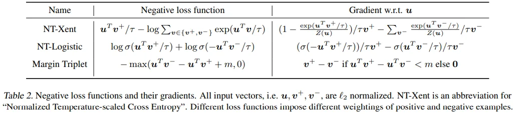
Table 2에서는 contrastive loss로 사용되는 logistic loss, margin loss를 NT-Xent loss와 비교했습니다.

• Input vector $u^{\intercal}$, $v^+$, $v^-$는 $l_2$ normalized 되어 있으며, $v^+$는 positive sample, $v^-$는 negative sample을 의미합니다.
• NT-Xent loss는 temperature로 scale된 (cosine similarity 같은) $l_2$ norm이 효과적이며, 적절한 temperature를 찾는 것이 hard negative의 학습에 도움이 됩니다.

• 다른 loss와 달리 NT-Xent loss는 cross entropy에 기반하기 때문에, negative sample의 상대적인 hardness를 학습에 반영할 수 있습니다. 그래서 공정한 비교를 위해, logitsic loss, margin loss에 semi-hard negative mining을 적용하여 모든 loss term이 아닌 semi-hard negative term의 gradient를 계산하도록 했습니다.

  • Semi-hard negative mining : FaceNet: A Unified Embedding for Face Recognition and Clustering (Schhroff et al. 2015)

• 모든 loss에 $l_2$ norm을 적용하였으며, hyperparameter search도 각각 수행했습니다.

  • Appendix B.10. Tuning For Other Loss Functions

    • 공정한 비교 및 실험의 간소화를 위해, negative sample에는 오직 1개의 augmentation을 적용했다고 합니다. (무슨 말인지 잘 모르겠습니다.)

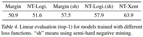
Loss 비교 실험의 결과는 Table 4에서 볼 수 있습니다.

• NT-Xent loss의 linear evaluation 성능이 매우 높은 것을 볼 수 있습니다.
• 그리고 margin loss와 logistic loss에 semi-hard negative mining을 적용했을 때 약 6 정도의 성능 향상이 있는 것도 확인할 수 있습니다.

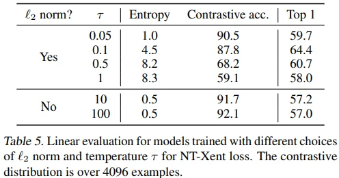
Table 5에서는 $l_2$ norm과 temperature $\tau$ 설정에 따른 linear evaluation 성능 차이를 보이고 있습니다. 흥미로운 점은 $l_2$ norm을 적용하지 않았을 떄, contrastive task accuracy는 오르지만 linear evaluation accuracy는 떨어지는 것입니다.

5.2. Contrastive learning benefits (more) from larger batch sizes and longer training

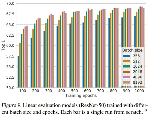
Figure 9에서 batch size와 epoch에 대한 실험을 진행했습니다.

• 작은 epoch에서 큰 batch size로 학습할 때 유의미한 성능을 보였고, epoch가 커짐에 따라 batch size 증가로 인한 이점은 점점 줄었습니다.

• 이는 supervised learning에서 큰 batch size를 사용할 때 성능이 하락한다는 내용을 다룬 Accurate, Large Minibatch SGD: Training ImageNet in 1 Hour (Goyal et al. 2017) 논문과 다른 양상입니다. 이에 대한 해석으로 저자들은 contrastive learning에서는 batch size가 클수록 (train epoch가 클수록) 더 많은 negative sample을 학습하여 수렴을 용이하게 한다고 합니다.

• Appendix B.1. Batch Size and Training Steps

  • 범용적인 결과를 얻기 위해 linear learning rate scaling을 적용했지만, 저자들은 LARS optimizer에 square root learning rate scaling이 매우 효과적임을 알아냈습니다. 특히, 작은 epoch에서 작은 batch size로 학습될 때 성능 향상 폭이 컸습니다. 결론적으로 batch size 8192 정도에서 saturate하는 양상을 보였고, epoch를 키우는 것은 여전히 유의미한 성능 향상을 보였습니다.

---

6. Comparison with State-of-the-art

• ResNet-50, ResNet-50(2x), ResNet-50(4x)

• Train 1000 epochs

Linear evaluation

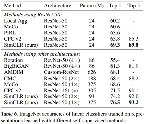
Table 6에서 linear evaluation 방식으로 성능을 측정했습니다.

• Appendix B.6. Linear Evaluation

Semi-supervised learning

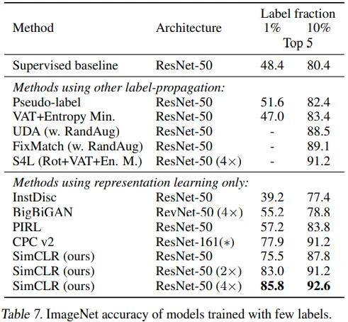
Table 7에서 class-balanced 방식으로 ImageNet의 1%, 10%를 선별하여 semi-supervised learning 성능을 측정했습니다.

• Appendix B.5. Semi-supervised Learning via Fine-Tuning

Tranfer learning

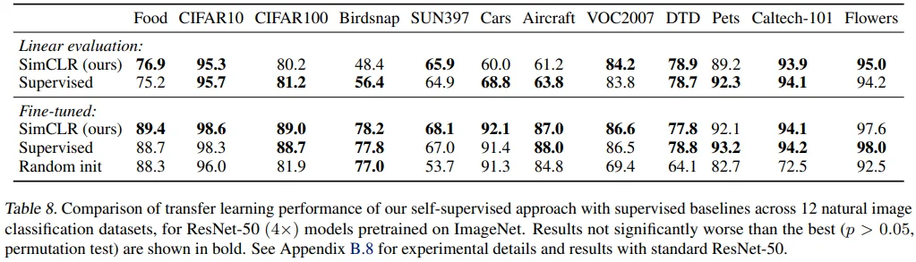
Table 8에서 ResNet-50(4X)의 12 datasets에 대한 transfer learning 성능을 측정했습니다.

• 각각의 dataset에 대한 hyperparameter tuning을 진행했고, validation 성능으로 hyperparameter를 선택했습니다.
• Linear evaluation : SimCLR 우세 (4) < Supervised 우세 (5)
• Finetuned model : SimCLR 우세 (5) > Supervised 우세 (2)
• Appendix B.8. Transfer Learning

---

7. Related Work

SimCLR 아이디어의 기반이 된 논문, semi-supervised learning 분야의 비슷한 논문, Handcrafted pretext tasks, Contrastive visual representation learning 분야의 논문들이 언급되고 있습니다.

• Appendix C. Further Comparison to Related Methods

  • 비슷한 시기에 나왔던 비슷한 논문들과의 자세한 비교를 하고 있습니다.
  • DIM/AMDIM, CPCv1/v2, InstDisc, MoCo, PIRL, CMC

---

Reference

• Paper