[논문리뷰] DPM: Deep Unsupervised Learning using Nonequilibrium Thermodynamics (ICML ‘15)

02 Oct 2023 in Papers / Review

arXiv link

github link

---

0. Abstract

반복적인 forward diffusion process로 data 분포를 파괴시키며, reverse diffusion process로 data 분포를 복원한다.

이렇게 함으로써, flexible하고 tractable한 생성 모델 학습이 가능하다. (학습이 빠르고, sampling이 용이하다.)

1. Introduction

Probabilistic 모델은 tractability와 flexibility가 trade-off 관계를 갖는다.

• Tractable: Gaussian, Laplace 분포와 같이 해석 측면에서 유용하지만 custom data 분포를 표현하기 어렵다.
• Flexible: custom data 분포에 fitting시키기는 용이하지만 tractable하지 못한 경우가 많다.
  • 이 경우 cost가 expensive한 Monte Carlo process를 통해 intractable 문제를 해결해왔음

1.1 Diffusion probabilistic models

기존 방법 대비 DPM이 갖는 장점은 다음과 같다.

• Flexible한 모델 구조
• 정확한 sampling
• 다른 분포와의 multiplication이 쉽다. (posterior 계산에 용이)
• Log likelibood, probability estimation cost가 expensive하지 않다. (Monte Carlo에 비해)

DPM은 generative Markov chain이다. (gaussian/binomial -> target data distribution)

• Gaussian 등 잘 알려진 분포로부터 sampling함으로써 tractability를 확보한다.
  • 매 step에서 small perturbation을 estimate하기 때문에, 한 번에 전체를 예측하는 것보다 tractable하다.
• Iterative diffusion process로 target data 분포에 fitting시킴으로써 flexibility도 확보한다.

1.2 Relationship to other work

기존 연구에서는 variational learning/inference로 flexibility를 챙기고, approximate posterior로 tractability를 확보했다. 이러한 연구들과 DPM의 차별점은 다음과 같다.

• Variational method보다 sampling의 중요성이 낮다.
• Posterior 연산이 쉽다.
• Inference/generation process가 same functional form이다. (예를 들어 VAE에서는 variational inference로 학습하고 reparameterization trick으로 sampling을 활용한 generation이 가능하게 하는데, 이러한 비대칭성으로 인해 challenging하게 된다는 관점?)
• 각 time stamp마다 layer를 두어 1000개의 layer를 가지며, 각각의 time stamp마다 upper/lower bound 정의 가능

Probability model을 학습했던 연구들은 다음과 같다.

• Wake-sleep
• Generative stochastic networks
• Neural autoregressive distribution estimator
• Adversarial networks (GAN)
• Mixtures of conditional gaussian scale mixtures (MCGSM)

Physics idea 관련 연구들은 다음과 같다.

• Annealed Importance Sampling (AIS)
• Langevin dynamics
• Kolmogorov forward and backward equation

2. Algorithm

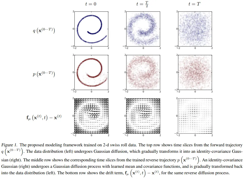
• 첫 번째 줄은 forward diffusion process를 의미한다. 2-d swiss roll data가 시간이 증가됨에 따라서 gaussian 분포로 바꾸어가는 것을 볼 수 있다.
• 두 번째 줄은 reverse diffusion process이다. Gaussian 분포로부터 원본 데이터 분포를 나름 잘 복원하는 것을 볼 수 있다.
• 마지막 줄은 각 time step에서 데이터 분포 평균의 변화 방향을 시각화한 것이다. t=T에서 t=0에 가까워질수록, 더 강하게 원본 2-d data 분포를 복원해내려는 모습을 볼 수 있다.

2.1 Forward Trajectory

학습할 데이터의 분포를 $q(x^{(0)})$라 하자.

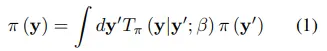
반복적으로 적용되는 Markov diffusion kernel을 $T_{\pi}(y{\mid}y{\prime};{\beta})$라 하면, 최종적으로 변화될 데이터의 분포 $\pi(y)$는 수식 1과 같이 정의할 수 있다. 여기서 $\beta$는 diffusion rate이다.

그리고 Markov diffusion kernel에서 y를 x와 t로 표현하면, forward process q와 의미상 동일해진다.

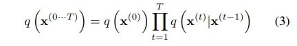
즉, markov 성질을 활용하여 forward trajectory는 수식 3과 같이 표현할 수 있다.

2.2 Reverse Trajectory

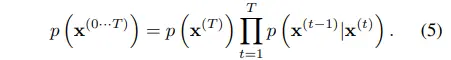
Forward trajectory와 같은 방식으로 수식 1을 reverse process로 표현하면 수식 5와 같다.

참고로 continuous diffusion에서 diffusion rate가 매우 작을 경우, forward process의 역연산이 identical functional form을 갖는 것이 증명되었다고 한다.

On the Theory of Stochastic Processes, with Particular Reference to Applications (Feller, 1949)

즉, forward process $q(x^{(t)}{\mid}x^{(t-1)})$가 gaussian/binomial 분포를 따르는 경우, 역연산인 $q(x^{(t-1)}{\mid}x^{(t)})$ 또한 gaussian/binomial 분포를 따른다는 내용이다. 이는 forward process q를 모방하는 reverse process p를 모델링할 수 있는 근거가 된다.

그리고 (아직 objectvie에 대한 언급은 없지만, forward를 모방하는) reverse trajectory는 gaussian 분포의 경우 mean/covariance를 예측하고 binomial 분포의 경우 bit flip probability를 예측하는 방식으로 학습한다. 즉, 상기한 값을 예측하는 cost * time이 training cost에 해당한다.

2.3 Model Probability

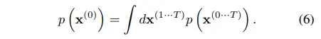
DPM의 목표는 원본 데이터 분포를 복원하는 것으로 $p(x^{(0)})$는 수식 6과 같이 표현할 수 있다.

수식 6은 intractable하기 때문에, 수식 3과 수식 5에서 정의한 forward/reverse trajectory를 대입하여 수식 7~9까지 전개한다.

• 이 과정에서 AIS와 Jarzynski equality로부터 힌트를 얻었다고 한다.
• Annealed Importance Sampling
• Jarzynski equality

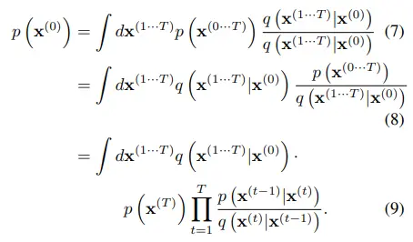
최종적으로 forward trajectory $q(x^{(1 \cdot \cdot \cdot T)}|x^{(0)})$로부터 sampling 한 번이면 된다.

• $p(x^{(T)})$은 초기값에 해당하고,
• p / q 꼴은 2.2에서 언급했던 것처럼 diffusion rate가 매우 작은 경우 forward/reverse 모두 gaussian 분포를 따르기 때문에 쉽게 연산이 가능하다.

저자들은 이러한 증명 과정을 두고 statistical physics 분야의 quasi-static process에 해당한다고 언급한다.

• Quasi-static process는 복잡한 문제를 단순화시켜 푸는 것을 의미하는데, 다음의 과정을 강조한 표현으로 생각된다.
• AIS와 유사하게, 현재 data 분포에서 시작하여 intermediate 분포를 거쳐 target 분포로 나아간다는 점
• Forward process와 reverse process가 동일한 분포를 따른다는 점

2.4 Training

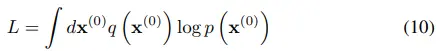
DPM은 log likeligood를 maximize한다. (따로 언급되어 있지는 않지만 cross-entropy 꼴과 유사하기에, forward process q를 target으로 reverse process p를 모델링하겠다는 접근으로도 보인다.)

이후 2.3의 수식 9를 대입한 다음,

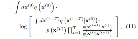
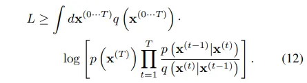
Jensen’s inequality에 의해 lower bound를 구할 수 있게 된다.

• $E[log(X)] \le log[E(X)]$ (log 함수는 concave)
• $E = E_{x^{(1 \cdot \cdot \cdot T)} \sim q}$
• $X = p(x^{(T)}) \Pi_{t=1}^{T} \frac{p(x^{(t-1)}{\mid}x^{(t)})}{q(x^{(t)}{\mid}x^{(t-1)})}$

이후 Appendix B에 의해 ELBO는 수식 13~14로 정리된다.

Forward/reverse trajectory가 동일하기에 수식 13에서의 equality가 만족한다. (KLD term이 0이 되면서 entropy term만 남기 때문에 equality로 보는 것으로 추측)

또한, (entropy term은 diffusion step과 무관하기에) ELBO를 maximize하는 것이 reverse process p를 모델링하는 것과 같아진다.

2.4.1 Setting the Diffusion rate B

Forward trajectory에서 diffusion rate $\beta_t$ 값은 중요하다. (AIS, thermodynamics에서도 그랬다.)

먼저 gaussian 분포의 경우, lower bound K에 gradient ascent 알고리즘을 적용하여 diffusion schedule을 학습한다. 이는 VAE와 마찬가지로 explicit한 방식이다. (참고로 first step인 $\beta_1$의 경우 overfitting 방지를 위해 작은 상수 값으로 설정했고, lower bound K의 미분 계산 과정에서는 diffusion rate를 상수로 설정했다.)

다음으로 binomial 분포의 경우, 매 step마다 1/T 만큼 diffusion한다. ($\beta_t = (T-t+1)^{-1}$)

2.5 Multiplying Distributions and Computing Posteriors

단순 inference는 $p(x^{(0)})$로 표현할 수 있지만, denoising같이 second distribution을 활용하는 경우에 posterior 계산이 필요하고 그러려면 분포끼리 곱할 수 있어야 한다. 이를 위해 기존 생성모델에서는 여러 테크닉을 적용했어야 한다.

반면 DPM에서는 second distribution을 단순 small perturbation으로 간주하거나, 아예 각 diffusion step에 곱하는 방식으로 손쉽게 해낼 수 있다.

• second distribution은 일종의 condition으로 생각됨
• $\tilde{p}(x^{(0)}) \propto p(x^{(0)}) r(x^{(0)})$

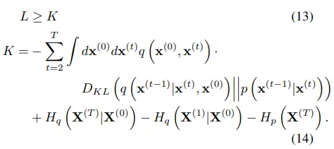
• (a): example holdout data
• (b): (a) + gaussian noise (var=1)
• (c): generated by sampling from posterior over denoised images conditioned on (b)
  • (b)의 noise를 reverse diffusion으로 제거하였더니 (a) 이미지와 유사하게 복원한다.
• (d): generated by diffusion model
  • (c)와 다른 이미지를 생성하는 결과로, init condition이 달라지면 다른 이미지가 생성됨을 보여준다.

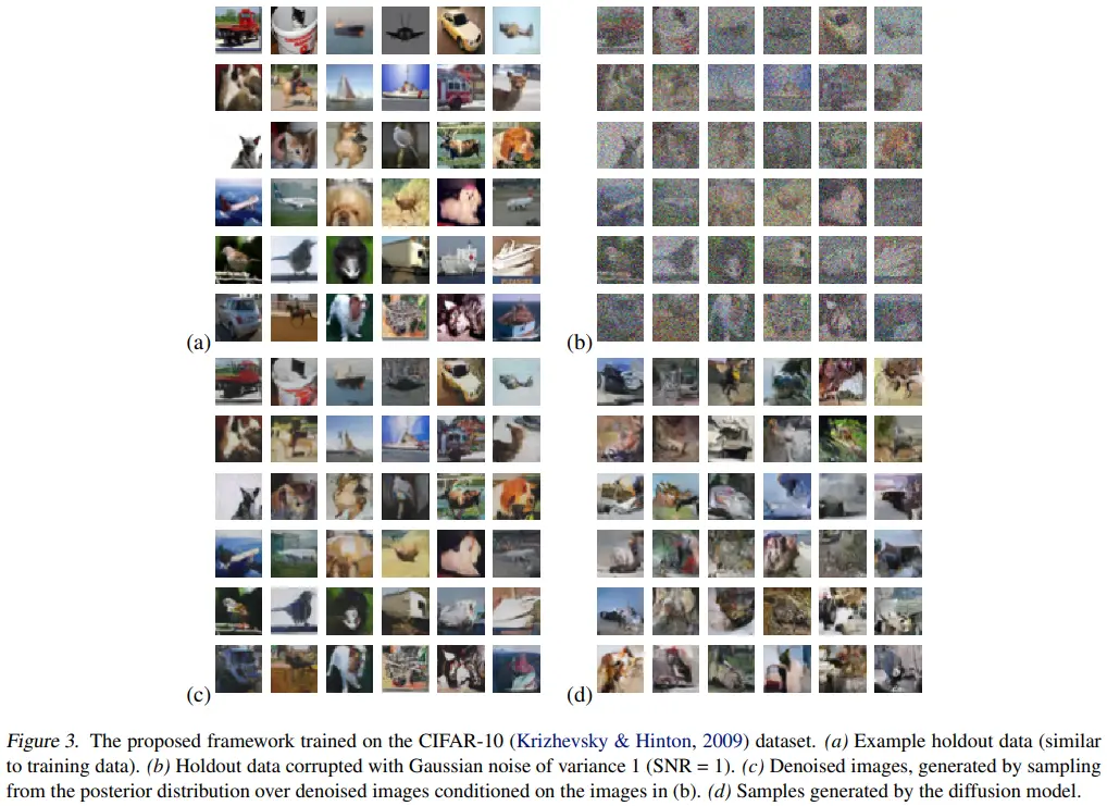
• (a): original
• (b): replaced with center gaussian noise
• (c): inpainted by sampling from posterior over noise conditioned on the rest of original
  • condition을 반영하여 center noise로부터 missing region을 생성한다.

2.5.1 Modified Marginal Distributions

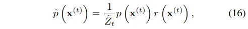
수식 16에 normalizing constant $\tilde Z_t$를 추가하여 modified reverse process를 정의한다.

2.5.2 Modified Diffusion Steps

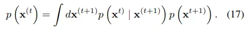
Reverse process의 markov kernel이 equilibrium condition을 따르기에, 수식 17로 표현할 수 있다.

더 나아가, 저자들은 modified reverse process에서도 equilibrium condition을 따를 것이라고 가정한다.

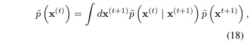
수식 16을 대입하고 정리하면 수식 19~20으로 전개할 수 있다.

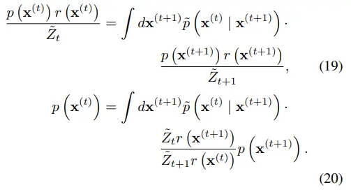
만약 수식 21이 성립한다면 수식 20을 만족할 수 있다.

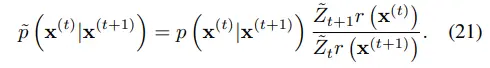
수식 21을 보면 gaussian 분포의 형태가 아닌데, 수식 16과 유사하게 표현하면 수식 22로도 나타낼 수 있다.

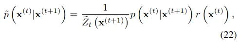
수식 22가 가능한 이유는 다음과 같다.

• $r({x^{(t)}})$는 small variance를 갖기 때문에, 수식 21에서 $\frac{r(x^{(t)})}{r(x^{(t+1)})}$을 small perturbation으로 간주할 수 있게 된다.
• Gaussian 분포에 대한 small perturbance는 mean에 관여한다. (자세한 증명은 Appendix C에서 다룬다.)
• Normalization constant는 잘 모르겠다. (수식을 완성하기 위한 constant라고 생각해서 큰 의미는 없어보인다.)

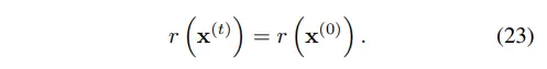
2.5.3 Applying r(x)

만약 $r({x^{(t)}})$가 충분히 smooth 하다면 reverse diffusion kernel에 대한 small perturbance로 간주할 수 있고, 이는 수식 22에서 설명하고 있다.

그 다음으로 $r({x^{(t)}})$가 gaussian/binomial 분포와 곱셈이 가능하다면 그냥 reverse diffusion kernel과 곱해버리면 된다. Inpainting과 같은 특수한 경우 $r({x^{(0)}})$에 대해서, noise가 없는 영역은 dirac delta function 개념을 도입하고 noise 영역은 constant로 설정했다고 한다.

2.5.4 Choosing r(x)

저자들이 step에 따른 scheuled r(x)도 실험해봤으나, constant로 두는 것 대비 이점이 없다고 판단했다.

2.6 Entropy of Reverse Process

Appendix A에 자세히 증명되어 있다.

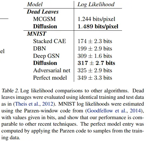
3. Experiments

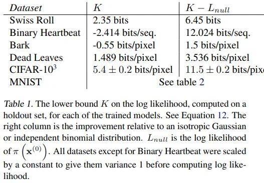
초기 데이터 분포의 영향을 제거한 K - $L_{null}$도 기록한 것이 인상적이다.

4. Conclusion

개인적으로 마음에 드는 문장을 인용하였습니다.

The core of our algorithm consists of estimating the reversal of a Markov diffusion chain which maps data to a noise distribution; as the number of steps is made large, the reversal distribution of each diffusion step becomes simple and easy to estimate.

Appendix

D. Experimental Details

D.2 Images

다음 figure는 이미지에 적용되었을 때의 모델 아키텍쳐이다.

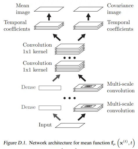
• Input image에 mean pooling을 통해 downsample한다.
• Multi-scale conv layer를 거친 feature map들을 다시 원본 사이즈로 upsample하고, 전부 더한다.
• 1x1 conv로 표현된 dense transform을 통해 temporal coefficient를 얻는다.
• 최종적으로 mean/covariance image를 얻는다.

위 figure에서 time이 관여하는 방식은 다음과 같다.

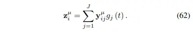
먼저 convolution output을 $y$라고 할 때, $y^{\mu}$는 평균, $y^{\Sigma}$는 분산을 위한 output으로 이해하면 된다. 이는 $z$에서도 동일하다. (1x1 conv를 거쳐 2 branch로 나뉘는 부분)

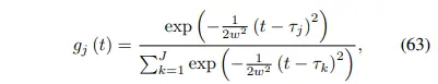
$g_j(t)$ 는 bump function은 softmax 함수 꼴이고, bump center인 $\gamma_k$는 (0, T) 범위를 갖는다. (이 과정을 어떻게 해석할지 잘 모르겠습니다. 다만 time이 관여하고 output이 확률 형태라는 점은 확실합니다.)

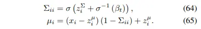
위에서 구한 $z^{\mu}$, $z^{\Sigma}$를 바탕으로 각 pixel i에 대한 $\mu_i$, $\Sigma_{ii}$를 예측할 수 있게 된다.