[논문리뷰] Context Cluster: Image as Set of Points (ICLR ‘23 Oral)

07 Oct 2023 in Papers / Review

arXiv link

GitHub link

OpenReview link

---

Abstract

CoC에서 정의하는 이미지란 정돈되어 있지 않은 points의 set이며, 간단한 clustering algorithm으로 featrue를 추출한다.

• 각 point에는 기존의 RGB뿐만 아니라 위치 정보(ex. coordi)가 추가된다. (5dim)
• Conv/Attention 대신 clustering이 spatial interaction 수행
• 디자인이 간단하기 때문에, 시각화를 활용한 해석력이 높다.
• 준수한 성능 (CoC를 더 복잡하게 만들면 더 성능을 끌어올릴 수 있다고 주장함)

1. Introduction

CNN에서 정의하는 이미지란 pixel들이 정돈되어 사각형 형태로 존재하는 것으로, local region에 적용되는 convolution operation으로 feature를 추출한다.

• Locality, translation equivariance와 같은 inductive bias 덕분에 효율적

ViT에서 정의하는 이미지란 patch로 이루어진 sequence이고, global range에 적용되는 attention mechanism으로 feature를 추출한다.

물론 각각의 장점인 convolution의 locality prior와 attention의 adaptive relationship을 융합하여 좋은 성능을 보인 논문도 있지만, 결국 CNN과 ViT의 융합일 뿐이다.

과연 convolution과 attention이 필수적일까? 아니다. Pure MLP-based, graph network(ex. Vision GNN)와 같은 접근을 보면 feature extractor의 새로운 패러다임이 될 수 있다.

CoC에 대한 설명은 다음과 같다.

• 모델링 과정에는 ConvNeXt, MetaFormer를 참고했다. (convolution, attention X)
• Point cloud analysis를 참고하여, CoC에서 각각의 pixel은 color에 position을 추가하여 5 dim으로 확장된다.
• Clustering 알고리즘은 SuperPixel과 유사하다.
• 다른 data domain으로의 일반화 성능이 준수하다. (ex. point clouds, RGBD image)
• Layer별 clustering 시각화를 통해 학습 양상을 파악하기 용이하다.

저자들은 이러한 접근이 이미지 전처리, segmentation을 제외하고 visual representation 관점에서는 유일하다고 주장합니다.

3. Method

3.1 Context Clusters Pipeline

From Image to Set of Points

• 1 point는 5 channel (RGB + coordi)로 이루어진다.
• 대부분의 도메인에서 data point에 feature/position 정보가 포함되기 때문에 CoC가 general하다고 저자들은 생각한다.
• Coordi는 이미지에서의 위치를 zero-mean이 되도록 표현하여, $\frac{i}{w} - 0.5$와 $\frac{j}{h} - 0.5$를 추가한다.

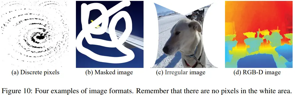
또한, figure 10에서 CoC의 input format은 중요하지 않고, input이 continuous하지 않아도 문제없다고 주장한다. (실험 X)

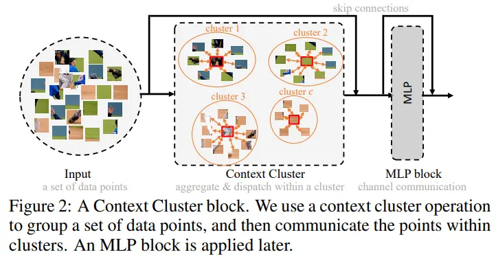
Feature Extraction with Image Set Points

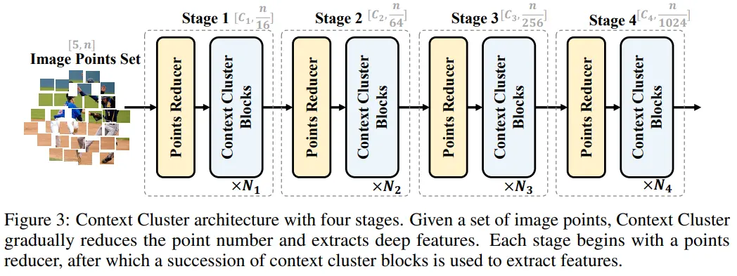
전체적인 아키텍쳐는 기존 모델들과 유사한 4 stage로 구성된다.

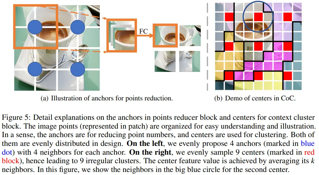
Left (point reduction)

• Blue circle은 anchor를 의미한다. (figure 상에서 4 anchors)
• Process
  • 각 anchor 주변의 neighbors는 channel을 축으로 concat된다.
  • FC(linear) layer를 거쳐 1개의 point로 fuse한다.
• Anchor 수를 고정했기 때문에 ViT에서 patch를 만드는 convolution layer와 유사하게 Conv2d로 구현했다.

Right (context cluster)

• Red blcok은 cluster의 center를 의미한다. (figure 상에서 9 centers)
• Center에 해당하는 point feature는 근처 feature들의 평균으로 정해진다. (figure 상에서 circle 내에 존재하는 point 9개의 평균이 center feature)

여담으로 저자들이 (어떤 값도 가능하지만) neighbors 값으로 4 또는 9를 사용하는 이유는 다음과 같다.

• 정사각 feature map을 형성할 수 있다. (detection, segmentation method에 적용하기 쉽다.)
• Conv, Pooling 등의 operation 사용이 용이하고 indexing search 작업을 피할 수 있다. (=코드 작성이 쉽다.)

Task-Specific Applications

• Classification: average all points of the last block’s output and use a FC layer
• Dense prediction (detection, segmentation): 일반적인 head를 사용하면 output points의 position을 rearragne할 필요가 있어서 CoC의 장점이 퇴색되는데, DETR과 같은 head가 CoC와 잘 어울릴 것이라고 주장한다.

3.2 Context Cluster Operation

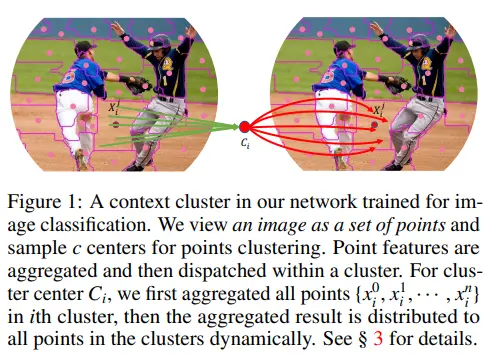
• Context clustering: 이미지에서 구역을 나누는 과정
• Feature aggregating: 초록선에 해당하며, cluster 내의 feature를 합치는 과정
• Feature dispatching: 빨간선에 해당하며, 합쳐진 feature를 cluster 내에 뿌리는 과정

Context Clustering

• Linear projection for similarity computation
• Propose c centers (center feature is computed by averaging its k nearest points)
  • AdaptiveAvgPool2d로 구현하여 center feature를 간단히 얻는다.
• Calculate the pair-wise cosine similarity matrix (between input and centers)
  • Pair-wise는 RGBxy 각각에 대해 적용된다는 뜻 (xy 덕분에 locality 특징 학습 가능)
  • cosine similarity matrix = centers * input = (B, M, C) * (B, C, N) = (B, M, N)
  • C = RGBxy = 5
  • M = local_centers = 4
  • N = points

Feature Aggregating

Dynamically aggregate all points in a cluster based on the similarities to the center point

즉, 위에서 구한 similarity를 활용하여, cluster 내에서 point들의 feature를 aggregate한다. (value space/value center라는 개념이 등장하는데, 추측으론 attention의 value를 차용한 것으로 보인다.)

• Linear projection for mapping to a value space
  • $v_i$ = index i에 해당하는 value space로 mapping된 point
• Propose v_c
  • Center c와 동일한 방식 (구현은 각각 한다.)
  • v_c와 normalized factor C의 분모에 있는 1은 학습 안정성을 위한 것이다. (1e-5처럼 낮은 값에서는 gradient vanishing 문제)
    • 만약 v_c가 없고 cluster에 어떤 point도 할당되지 못하면, C가 0이 되어 학습이 불가해진다.
• Similarity
  • $s_i$ = index i에서의 similarity 값
  • $\alpha, \beta$ = learnable scalar (scale and shift)
  • $sig$ = sigmoid function
    • Similarity를 (0, 1)로 re-scale하는 효과
  • 이러한 방식이 similarity를 그대로 사용하는 것보다 효과적이다.
    • 이미 동일한 cluster에 속하기 때문에 similarity가 불필요하게 높아 학습 효과가 낮은 것으로 추측된다.

Feature Dispatching

The aggregated feature g is then adaptively dispatched to each point in a cluster based on the similarity

• Similarity
  • Feature aggregation과 동일하게 처리된다.
• Projection(FC)
  • Value space dim -> original dim
• $p_i$ = index i에 해당하는 point로, 위 식을 통해 point가 update된다.

Multi-head Computing

위 프로세스는 attention과 유사하게 multi-head 연산이 가능하며, 실제 성능 향상에도 도움이 된다. (table 2 참고)

3.3 Architecture Initalization

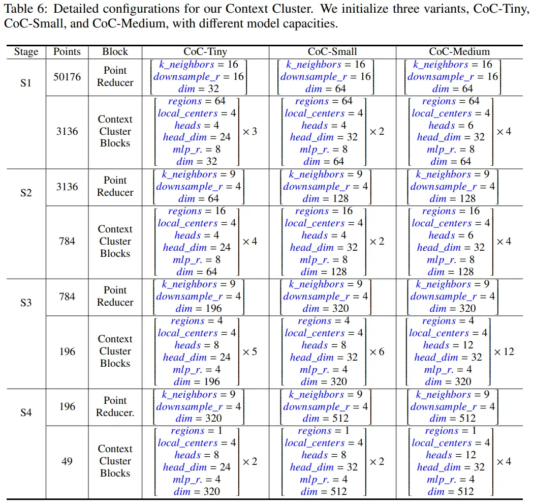
• Point Reducer: k_neighbors만큼 fuse하고, downsample_r만큼 point 수를 줄여나간다. (+ output dimension 조절)
• Context Cluster
  • regions: 하나의 local region이 몇개의 포인트로 이루어지는지 (저자들은 49 points를 1 region으로 간주함)
  • local_centers: 하나의 local region에 몇개의 center가 포함되는지 (저자들은 4 centers로 고정함)
• 이러한 design이 유일한 것은 아니다. CoC-Tiny variation은 아래 방식을 사용한다.
  • region partion: [49, 49, 1, 1]
  • region centers: [16, 4, 49, 16]

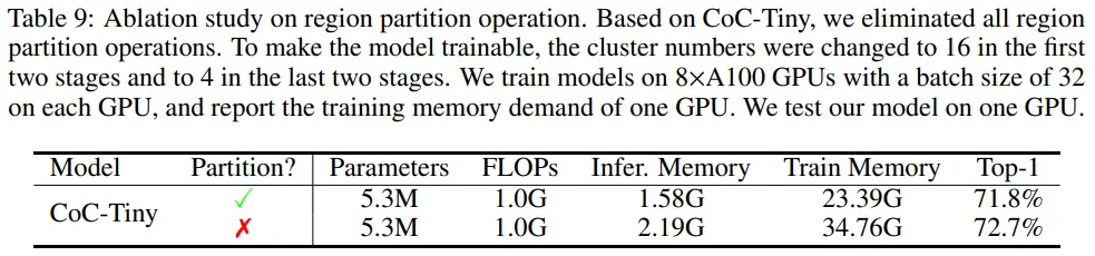
CoC에서 (Swin Transformer와 유사하게) region partition을 적용한 이유는 연산 비용 때문이다.

• Region partition이 locality에 대한 inductive bias를 제공하지만, 모델의 global interaction이 희생된다.
• Table 9을 통해, 모델의 global interaction이 CoC 성능 향상에 중요하다는 것을 확인할 수 있다.

3.4 Discussion

Fixed or Dynamic Centers for Clusters?

Fixed cluster center를 사용함으로써 inference 연산 비용을 낮출 수 있다.

• CoC-Tiny 모델의 dynamic center ablation 실험 결과, 71.83% -> 71.85%로 성능 향상이 미미했다. (Appendix)

Overlap or Non-overlap Clustering?

Point cloud analysis의 철학과는 다르게, CoC는 point에 오직 1개의 center만 할당한다. (non-overlap)

물론 성능만 보면 overlap이 더 좋을지도 모른다. 하지만 CoC에서 overlap은 본질이 아니며, 추가되는 연산 비용 또한 불필요하다고 판단했다. (그리고 non-overlap이 simple하다.)

4. Experiments

4.1 Image Classification on ImageNet-1k

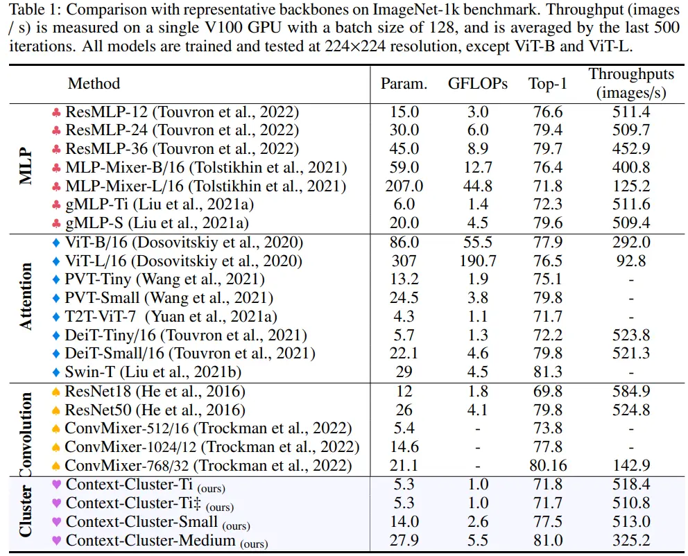
SOTA에 준하는 성능은 아니지만, clustering 알고리즘이 convolution/attention과 비교될 만한 feature extraction 방식임을 확인할 수 있다. 또한, 저자들은 MLP-based 모델보다 성능이 높은 점을 근거로 CoC가 단순 MLP-based 모델에 해당되지 않는다고 주장한다.

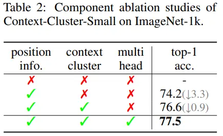
CoC-small의 ablation study이다. (Appendix)

• Position info.(x): untrainable

4.2 Visualization of Clustering

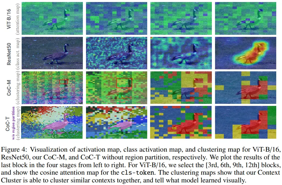
• 가장 우측인 4th block을 보면, goose를 하나로 인식하면서, backgound 영역도 넓게 clustering한다.
• 1st/2nd blcok의 red box를 보면, 초기 stage에서도 goose neck을 성공적으로 clustering하고 있다.

4.3 3D Point Cloud Classification on ScanObjectNN

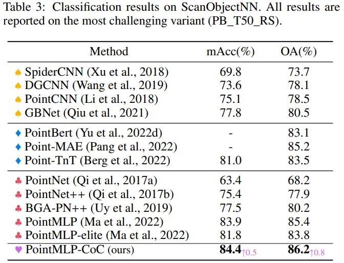
PointMLP를 base로 하는 PointMLP-CoC의 결과를 보면 꽤 성능이 향상된다.

• Residual Point Block 앞에 Context Cluster block을 삽입했다.
• Multi-head가 아닌 one-head의 결과로, multi-head 사용 시 성능 향상이 기대된다고 주장한다.

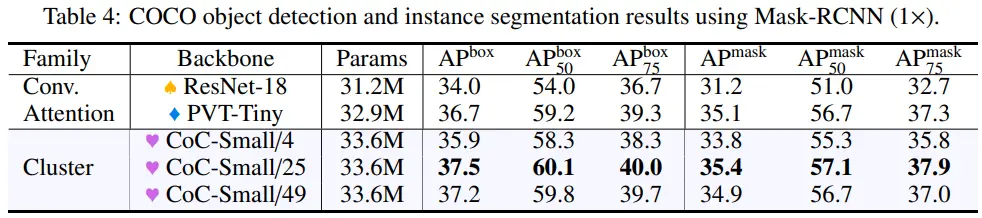
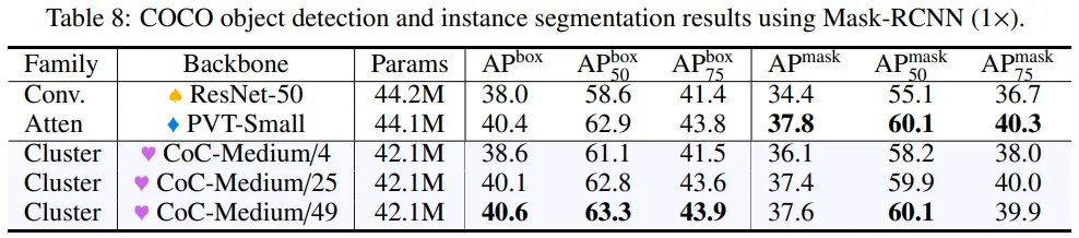
4.4 Object Detection and Instance Segmentation on MS-COCO

• Classification에서 49 points, 4 local centers 사용
• Detection/Segmentation에서 1000 points, 4 local centers 사용 (이후 4에서 25, 49 centers 까지 확장)

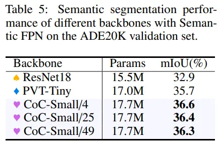
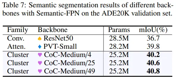
4.5 Semantic Segmentation on ADE20K